Search This Blog

Tuesday, May 28, 2013

26 Introduction to Variation

W. Edwards Deming, the famous quality improvement guru, claimed that the two most important things for managers to understand are:
1.     Variation and how to deal with it
2.     The forces that motivate and demotivate people
The subjects of the first 21 lectures, motivating, staffing and communicating, address the forces that motivate and demotivate people, i.e. the Theory Z portion of effective leadership. Forces mean the collection of perceptions, understandings and misunderstandings that influence the attitude and behavior of people. Lectures 23 – 25 introduced management of processes, part of the control function of managers, and treated the stand alone topics of managing risk and theory of constraints. Now we turn to variation and how to deal with it, the central theme of process improvement and process control. Managing in the presence of variation is also part of the control function of managers.
W. Edwards Deming claimed that the inability to interpret and use the information in variation is the main problem for managers and leaders. (See the book Out of the Crisis by W. Edwards Deming) When there is a problem with any work process the manager and the employees both must understand when the manager must act and when employees must act. It is through an understanding of variation and the measurement of variation that they understand when and who should take action and, just as importantly, when not to take action. Thus variation is involved in both improving poor processes and maintaining good processes.
Variation is just the reality that actual values of parameters, physical or financial, have some statistical spread rather than being exactly what we expect, specify or desire. For example, we may have a budget for supplies of $1000 per month. When we look at spending for each month it is typically close to but not exactly $1000. Over time the spending might look like that shown in figure 15.


Figure 15. An example of variation from planned budget by actual spending.
For our purposes the definition of variation is deviation from planned, expected or predicted values of any parameter. The parameter might be financial, as in the example shown in figure 15, it might be in units of production per day or minutes per service, or it might be a physical parameter, such as the dimension of a machined part. Thus variation occurs in all the work processes of any kind of organization. Therefore, as Deming implied, the effective leader must understand the information in variation and how to properly manage in the presence of variation.
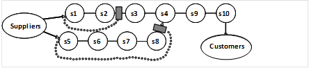
Let’s start by returning to the work process illustrated in figure 12, the SIPOC diagram.  Where might we expect to see variation in a work process? The answer is everywhere. Deviations from ideal inputs are variation. Deviations from ideal outputs are variation. Deviations from expectations in use are variation. Variation in use can be due to either hidden variation in outputs or unexpected variation in the use environment or the use process.
Let’s define an effective process from a customer’s point of view. It is a process that produces outputs that meet or exceed the customer’s expectations for quality and cost. Customers can be internal or external to the enterprise or the organization that owns the process. Customers have stated and unstated expectations. Specifications, requirements, standards, and contract items are examples of customer’s stated expectations. Customer’s unstated expectations are typically suitability for all conditions of use and affordability. Therefore, for the purposes of process improvement discussions, we can say that an organization’s effectiveness is determined by the effectiveness of its processes in satisfying its customer’s expectations. (In general the effective organization must satisfy all its stake holders’ expectations, including managers, workers, owners and the community as well as the customers.)

Variation Drives Process Effectiveness

We can see the effects of variation by examining an ideal business process (figure 12, an ideal process is repeated in the top half of figure 16) and a typical process as shown in the bottom half of figure 16.


Figure 16. Comparison of a typical process to an ideal business process.

An ideal process converts all of the supplier’s inputs to outputs that satisfy the customer’s expectations. A typical process includes inspection steps to ensure that a defective input is not sent to the process or a defective output is not sent to the customer. The customer also adds an inspection step because of receiving defective outputs in the past. If outputs fail any of these inspections the failed item is scrap or must be reworked. It’s easy to see that the typical process is more expensive, and therefore less effective, than an ideal process because inspections cost money and scrap or rework cost money. In a typical chain of processes costs of failing inspection increases as the work progresses along the chain because more rework is required if an inspection is failed at processes near the end of the chain. Thus often the largest cost to the organization is warranty costs from customer returns. That is the reason for the inspection of the outputs before they are sent to the customers. The reason these inspection steps are added is the presence of variation. If there was no variation in the inputs or the outputs then there would be no need for inspection to find those items whose variation from ideal is larger than acceptable.
Notice that even the ideal process has inputs and outputs that exhibit variation but for the ideal process this variation is within acceptable limits most of the time. We need to define what we mean by “most of the time”. If there is variation then sooner or later a product will fail to meet customer expectations if there is no inspection. (Actually it will happen even with inspection since no inspection is perfect, i.e. inspection is a process that also has variation.) If the variation is small enough so that only rarely is there a customer return and the cost of correcting this return plus the cost of the disgruntled customer is less than the cost of including inspection then it makes business sense to not have inspection.
Now I hope the student is thinking that to make a valid decision to not include inspection takes data to establish that the variation is sufficiently low. The astute student is also thinking that collecting such data costs money also, perhaps as much as the inspection. This is an example of what is meant by a manager needing to know how to manage in the presence of variation. Next we examine how a manager can achieve such understanding and make good decisions in the presence of variation.

Variation is a Statistical Phenomenon

To understand managing in the presence of variation we must answer the questions how can the manager decide:
·       when to take action,
·       what action to take and
·       who should take the action?
Managing correctly in the presence of variation requires the use of methods based on statistics since variation is a statistical phenomenon. The statistics needed for 85% or so of a manager’s work is relatively simple and easily learned. The effective leader and all workers must understand and use these simple methods. However, there are situations that require more elaborate statistics. Every organization should have access to at least one person well versed in statistical methods so that managers and process improvement teams have a resource to check their work and assist on complex problems. This statistical expert can be a consultant or a worker that is well trained in statistics.
Here we are going to briefly look at some of the most important simple methods. As an example, figure 17 illustrates the daily averages of phone expenses for an organization plotted for each month of a year.


Figure 17 A graph of an organization’s daily phone expenses averaged for each month of a year.
Should the manger take action in response to the March expenses? The June expenses? If action is necessary in response to the March expenses, whose action is it? The manager’s? The workers? If the manager is expected to discuss unusual expenses in a weekly or monthly report what should the manager say about the March and June expenses?
Control charts are a visual method of answering the questions posed about the phone bills. A control chart for the phone expenses data from figure 17 is shown in figure 18. You can learn how to generate control charts later. For now I only partially describe how to interpret the data in a control chart.


Figure 18 A control chart for the example phone expense data.
The line with diamond markers is the same data shown in figure 17. The line with the square markers results from averaging the data over a whole year. The line with the triangle markers shows the range of variation of daily expenses for a given month. The two lines labeled Upper CL and Lower CL are upper and lower control limits, which are statistically determined from the data set. For the purposes of this introduction it isn’t necessary to know how to calculate the control limits. The control chart tells us that, with the exception of the March data point, the phone expenses are stable, that is they exhibit variation about a stable sample average, which is not steadily increasing or decreasing. A stable process is predictable, e.g. frequency of errors, efficiency, process capability and process cost are predictable. Deliberate changes to a stable process can be evaluated.  Note that some process improvement literature refers to a stable process as being “in control”.
Variation exhibiting a stable statistical distribution is due to the summation of many small factors and is called common cause variation. Changes to a stable process, i.e. one with common cause variation is typically the manager’s responsibility but can be the responsibility of trained and empowered workers. Knowledge workers should be responsible for common cause variation because they are usually more expert with respect to their processes than their managers. However, as is described in the next lecture, even knowledge workers should not be empowered to control their processes before they have been trained in statistical methods because mistakes can make processes worse.
Only the data point for one month, March, falls above or below the two control limit lines. Variation that is outside the stable statistical distribution, i.e. above the upper control limit or below the lower control limit, is special cause variation.  The point for March falls below the lower control limit. This means that the March data is special cause variation. Special cause variation is the workers responsibility; they typically know more about possible causes than the manager because they are closer to the process. But the workers need training in problem solving to fix special cause variation and they need to be empowered to make fixes to their processes.
The workers should review the data for March and examine the phone system to see if they can determine the reason the daily averages were so low. For example, the phones may have been out of order for a week, which would have lowered the daily expenses but require no action other than getting the system operating again. Properly trained and motivated workers can handle special cause problems, usually without any management involvement.
A stable process is a good candidate for process improvement. The goal of process improvement for a stable process is to reduce the variation and/or change the mean. Process improvement should not be attempted on a process that is unstable until the process is brought to a stable condition because changes in data taken on an unstable process cannot be uniquely attributed to the action of the process improvement. The special cause variation that makes the process unstable must be removed before beginning process improvement.
Note that the control chart also provides the manager information useful in considering process improvement. In the example shown in figure 18 the yearly average phone expenses are about $21 per day. A manager can evaluate the cost benefit of making a change to the phone service based on this data since it is stable over a year. If the manager can make a change without investment that promises a 10% reduction in phone expenses the manager can see that data will have to be monitored for about four to six months to determine if the mean daily expenses do indeed drop from $21 to $19 because the normal range of variation in monthly averages is larger than the expected change. However, if the change really works as promised then in about four to six months the monthly averages should begin to vary about a new long term average and the control chart will show this change.

Exercise

1.     Go to “Control Charts” in Wikipedia (http://en.wikipedia.org/wiki/Control_) and read the article. This material expands upon the introduction given in this lecture.
2.    Go to http://www.goalqpc.com/shop_products.cfm and buy yourself a copy of Memory Jogger II. This handy book teaches everything you need to know about problem identification and problem analysis. It is small enough to carry in your pocket and it is your guide to the details of process improvement. If you prefer a spiral bound version it is available from Amazon.com (Michael Brassard, and Diane Ritter, The Memory Jogger II: A Pocket Guide of Tools for Continuous Improvement and Effective Planning) There is also a Six Sigma Memory Jogger available.
The Memory Jogger book recommended here is so widely used and so effective for the practical user that there is no point in repeating the material in this course. The student is expected to study the Memory Jogger and put the techniques into practice. This means that the student and all the people reporting to the student are to have the Memory Jogger book , or an equivalent, be trained in the techniques summarized in the book and put these techniques into practice. This is essential if an effective organization is expected. The exception is if your organization is following the Six Sigma approach where only selected people are highly trained.
If you prefer not having to learn statistical techniques yourself you can attend training if your budget and schedule permits. One example workshop in statistical process control is offered by the American Supplier Institute. See: http://www.amsup.com/spc/1.htm. This workshop focuses on manufacturing but the techniques work for any type of organization. A web search reveals many other training organization offering similar programs. I have found it more cost effective when training all workers to bring the trainer to the organization rather than sending workers to outside training.

If you find that the pace of blog posts isn’t compatible with the pace you  would like to maintain in studying this material you can buy the book “The Manager’s Guide for Effective Leadership” in hard copy or for Kindle at:
or hard copy or for nook at:
or hard copy or E-book at:


Wednesday, May 22, 2013

25 Overview of Theory of Constraints

The theory of constraints involves techniques for improving processes that have to be learned independently of the material we address in subsequent lectures. This theory should be applied to business processes before beginning the process improvement methods that are discussed in the following lectures. If the student understands the theory of constraints and if this theory is being applied to the business processes the student is concerned with then this lecture can be skipped. If not, this overview introduces the theory and gives the student some feeling for the necessity for learning and using this theory.
Theory of constraints deals with aspects of control often neglected or wrongly presented in standard texts. I suspect the likely reason is that theory of constraints as applied to business organizations was made popular outside of business schools by a physicist, Eliyahu M. Goldratt. Theory of constraints is described by Goldratt via his books The Goal, The Race, Critical Chain & other process oriented management books. These books are “business novels” and enjoyable reads as well as being excellent self-training books. Theory of constraints is appropriate to processes associated with manufacturing operations, back and front office service operations and projects. I distinguish between back and front office service operations because although theory of constraints applies to front office service operations it shouldn’t be the main focus when dealing directly with customers. This is because it is better to be effective with customers than to be highly efficient at the expense of some effectiveness.
Theory of constraints is based on the fact that the throughput of a process can be no greater than the throughput of the slowest step in the process, i.e. the constraint. It is a simple and seemingly obvious concept but having seen many offices with desk after desk stacked with paper work waiting to be processed and many factories with work in process stacked around machine after machine I can tell you that it isn’t obvious to many managers in spite of the fact that violating this theory leads to inefficient operations and excessive costs.
A basic work process, applicable to any organization, is shown in figure 12.


Figure 12 A basic work process has suppliers, inputs, outputs and customers.
This chain is often called SIPOC after the initials of each element in the chain. Manufacturing, project and back office service processes are typically many step processes, each with suppliers, inputs, outputs, & customers. A simple example with ten steps is shown figure 13. Each circle with an S is a SIPOC chain in which the preceding S is the supplier of inputs to the S and the following S is the customer for its outputs. Note that a process can have more than one supplier, as S4 is supplied by S3 and S8 in this figure. Similarly a process can have more than one customer. A more complex, but typical process might have loop backs where material or paperwork not meeting standards is sent back to an earlier process for rework.


Figure 13 Typical business processes integrate many individual SIPOC processes.
If we assume that each of the steps shown in figure 13 has a different through put then the theory of constraints states that the through put of the overall process cannot be any larger than the through put of the slowest step. If the manager in charge of an overall process like that illustrated in figure 13, with each step having a different through put, expects the workers to stay busy you can imagine what results. Work in process (WIP) builds up in from of all steps that are slower than the previous step. This excess WIP can lead to several problems, including:
·       In manufacturing operations and in some project operations the WIP leads to excess inventory costs.
·       Associated with excess WIP is excess cycle time, i.e. the time from the first step to the final step in the overall process.
·       If a worker at one of the non-constraining step begins to make errors in paperwork or if a machine at a non-constraining step begins to produce defective parts then excess costs result from the extra rework required on all the defective material produced before the problem is detected at some subsequent step
·       Eventually expediters and/or overtime are added to ensure that time critical work is located and processed at the expense of other less critical work, leading to excess labor costs.
A second, and again often overlooked, result of the theory of constraints is that there are no additional costs incurred if workers at non-constraining steps are idle as long as there is material available for the worker or machine at the next step. This means that if such workers are cross trained then they can do other productive work when there is a buffer of output work after their step. The value of workers doing other work justifies paying premium wages to workers that are cross trained and the cost of cross training.
Most important is that workers at non-constraining processes have time to spend on process improvement and, since total productivity is not reduced, there is no additional cost for the process improvement labor. This is one reason theory of constraints should be applied to work processes before initiating other process improvement activities.
Figure 14 illustrates how to control processes with a constraining step.


Figure 14 Adding buffer inventories and controlling work material release controls work in process for processes with constraining steps.
In the example shown in figure 14 step 3 is assumed to be the constraining step. Buffer inventory is maintained in front of step 3, indicated by the small rectangle, so that it can never be idle due to lack of input. The size of the buffer in front of step 3 is controlled by the rate of work material released to the input of step 1, indicated by the dotted line from the input of step 1 to the buffer inventory at the input to step 3. It is also correct practice to add a buffer in front of step 4 and regulate the input to step 5 to control the size of this second buffer. The reason for the second buffer is to ensure that step 4 does not become the constraining step due to material not being available from step 8. Note that this process control approach applies to any type of business that involves material, i.e. paper, electronic media or parts, moving from step to step to accomplish an overall work objective.
A personal experience is a good illustration of the problems caused by not applying the theory of constraints. I was asked to consult for a factory that was in danger of being shut down and the work moved out of the country because the corporate office was not satisfied with the factory’s performance. A quick tour showed that there was excess WIP nearly everywhere. In fact a special material handling system had been installed just to deal with the partially finished goods throughout the factory. A few questions revealed that the constraining process was the final process before the products were boxed and shipped.
I held a Saturday training system for the managers. I asked them what the cycle time was for their products. They answered that it was about 35 days from first material release to shipping products made with that material. I then asked what the cycle time would be if material moved from process to process with no waiting time in front of each process. They thought awhile and answered that it would be 7 days. A few more leading questions and I could see light bulbs coming on in a few minds and excited expressions on faces. Incidentally, the first person that comprehended what they had been doing wrong was a woman doing administrative work in the front office. By Monday they had plans worked out to change their methods and were starting to implement the plans.
I called the general manager a couple of months later and asked if the cycle time had changed. They had two products going through the same production line. He said the cycle time for one product had been reduced to the ideal 7 days by applying theory of constraints. They began releasing material into the line at the rate of the final constraining process and maintained buffer work in process only in front of the constraining process. Unfortunately, he was not allowed to control the release of material for the second product and its cycle time was still about 35 days. Corporate marketing people controlled the release of material for the second product and they released it according to their sales instead of the factory capabilities. I never learned if the general manager was able to convince corporate management that marketing’s control of material release for the second product was the cause of the factory’s excess cycle time, excess WIP and associated excess costs.
This short introduction to the Theory of Constraints illustrates the principle. Managers of manufacturing or back office service operations should study Theory of Constraints, just in time (JIT) inventory control and Lean techniques and understand the value of small lot size in controlling the cost of poor quality. Project managers should study critical path scheduling as well as the theory of constraints. I recommend project managers read Goldratt’s book Critical Chain, which addresses scheduling for projects.

Exercise

Like lecture 23 this lecture is only an introduction and no exercises are required unless the student isn’t familiar with the theory of constraints and using it already. If the student isn’t knowledgeable in these techniques and isn’t already using them then additional self-study is necessary to learn how to put them into practice for real business processes, which tend to be more complex than the simple example used here to illustrate the principles involved. I recommend reading Goldratt’s books because they are fun reads as well as excellent for self-training.

If you find that the pace of blog posts isn’t compatible with the pace you  would like to maintain in studying this material you can buy the book “The Manager’s Guide for Effective Leadership” in hard copy or for Kindle at:
or hard copy or for nook at:
or hard copy or E-book at:


Monday, May 13, 2013

24 C The Risk Burn Down Chart


A spreadsheet similar to the risk register can be developed to manage risks and manage the budgets associated with risk management on large and long duration projects. It isn’t possible to avoid all arbitrariness in forecasting the risk management budget but it is possible to provide good management visibility into the process. One approach is as follows: (This description is a bit tedious so look ahead at figures 10 and 11. If the process is obvious to you from the figures skip the text. If not then just wade through the description. It may help to drawn out the spreadsheet as you read the description.)
•           Develop a spreadsheet with time, e.g. months, in the first column and the known risks in the first row of adjoining columns. The planned mitigation expense estimate as a function of time for each risk is added in the rows for each known risk. Summing the entries in each row across columns results in the estimated mitigation expense for all risk mitigation activities for that time period. As new risks are identified they are added in the first row of new columns and mitigation budgets are added in appropriate time rows in the new columns.
•           Develop a second spreadsheet with the following columns
o          Time line, e.g. month number from beginning of the project or actual dates
o          Planned Mitigation Expense per time period to be spent on risk mitigation for known risks, i.e. the cumulative value of the row for that time period from the first spreadsheet
o          Cumulative Planned Mitigation Expenses, i.e. the cumulative cost estimates for mitigation activities for the risks known at the time the plan is developed.
•           Recognize that as the project progresses new risks will appear as decisions are made and additional risk management budget is needed to mitigate these new risks. Therefore add the following columns to the spreadsheet.
o          Adjusted Cumulative Mitigation Budget; the planned expenses plus an adjustment, e.g. an arbitrary percentage, to mitigate unknown risks that will arise during the project.
o          Actual Mitigation Expenses for each time period.
o          Cumulative Actual Mitigation Expense
It may be helpful at this point to show a chart resulting from an example of the process described so far. Figure 10 is a chart for a large project in which the mitigation budget is nearly $40 million dollars. In this example the initially identified risks were planned to be mitigated with just over $30 million. The arbitrary adjustments for unknown risks increased the budget to nearly $40 million and the actual expenses at the end of a year were just below the adjusted budget. For situations where the budget for risk mitigation is released incrementally or for a large project that continues for several more years having data such as this chart provides the project managers sound arguments to defend their requests for risk mitigation budgets.

  Figure 10 An example of risk mitigation budget and expense resulting from the example approach.
The mitigation budget and expense are only half of the story. Risk is the rest of the story so now let’s return to the example approach:
•           At the beginning of a project sum up the expected values of all risks on the risk register. This cumulative risk value is the amount of over budget expense that is likely if initially known risks are not mitigated before they impact the project. Add a column to the second spreadsheet for this Cumulative Risk Value before Mitigation.
•           Add a risk value adjustment factor for each time period to cover unknown risks that will arise and add a new column to the second spreadsheet for the Adjusted Cumulative Risk Value before Mitigation. These “adjusted” values represent the best estimate of how both identified and new risks will be mitigated throughout the project
•           As the project continues, new risks are added and all risks are mitigated so that a Cumulative Risk Value after Mitigation can be added to the spreadsheet. Now there is sufficient data to construct a Risk Burn Down Chart which shows how the risk value is reduced over time by the risk mitigation work.
An example of a risk burn down chart is shown in figure 11. In this example the adjusted and actual cumulative risk values track each other reasonably well. If the manager of this project needed additional risk management funding in the middle of the project then showing this chart to the funding authority would provide excellent justification for the needed funds. If the planned and actual risk mitigation expenses also tracked each other well, as in the example shown in figure 10, then the funding authority should have good confidence in the management team.

 Figure 11 An example risk burn down chart for a large project with high initial risk.
The charts resulting from the approach outlined above are useful for showing those responsible for funding projects the most likely project expense if risk mitigation is effectively conducted and the likely budget impacts if risks are not proactively mitigated. In the example shown the likely budget impact if risks are not mitigated is over $400 million. This budget impact is reduced to about $23 million by an expenditure of about $38 million for a total impact of about $63 million compared to over $400 million.
The percentage adjustments risks that will be identified during a project are necessarily arbitrary but can be adjusted during the project if the actual expected risk value line deviates substantially from the adjusted expected value line.
In summary, spending a small amount of money in proactively mitigating risks is far better than waiting until the undesirable event occurs and then having to spend a large amount of money fixing the consequences. Remember that risk management is proactive (problem prevention) and not reactive. Also risk management is NOT an action item list for current problems. Finally, risk management is an on-going activity. Do not prepare risk summary grids or risk registers and then put them in a file as though that completes the risk management process, a mistake inexperienced managers make too often.
Exercise
1. Spend some quiet time thinking about what the worst possible thing your competitors could do that would negatively impact your organization in the short and long terms. If you have already done this and have mitigation plans in place or on the shelf you are a mature risk manager. If not, you have some homework to do.
2. Handling anything your competitors do or responding to the loss of your most important customer are the easy ones. Now imagine that your organization is stable, progressing well on improving effectiveness, trust in management is growing, enthusiasm is growing and then your superiors tell you to lay off 10% of your people in order to increase enterprise profits for the year. You know this is going to demoralize the organization for some time and erode trust in the benefits of working to improve the organization. How do you respond to your people and to your superiors? There is no easy answer to this question but in today’s environment it is not an unlikely occurrence and you should be prepared for it.
2. Does your organization have a standard risk management process in place? If so then go on the next lecture. If not then think through a plan to put a standard process in place and train workers to use it. This can be a commercial process or a process you or your workers develop. You can implement it via formal training or on an incremental basis. The important thing is having a process and using it religiously.

If you find that the pace of blog posts isn’t compatible with the pace you  would like to maintain in studying this material you can buy the book “The Manager’s Guide for Effective Leadership” in hard copy or for Kindle at:
or hard copy or for nook at:
or hard copy or E-book at:


Tuesday, April 30, 2013

24 B The Risk Register


The risk register ranks risks by the dollar value of each risk according to the operational definition of risk given earlier. Constructing the risk register on a spreadsheet allows risks to be sorted by dollar value so that the highest risks are always on top of the list. The risk register also facilitates keeping all risks in the same data base even though management actions may be active on only the top five or ten at any time. When a high risk is mitigated the expected dollar value of the risk is reduced and it falls out of the top five or ten but is still on the list. This enables reviewing mitigated risks to ensure they remain mitigated or to readdress a risk at a later time when all the higher risks have been mitigated to even lower values. An example of a simple risk register constructed on a spread sheet is shown in figure 9.


Figure 9.  An example template of a risk register constructed in columns on a spread sheet.
The risk type and impact if risk occurs are usually described as “if”, “then” statements. This helps the management team remember specifically what each risk entails as they conduct reviews over the life of the activity. Expected values are expressed in dollars, which facilitates both ranking and decisions about how much resources should be assigned to mitigation activities. I am assuming of course that in managing activities in your organization it is the practice to hold some fraction of the budget in reserve to handle unforeseen events. It is this reserve budget that is assigned to risk mitigation activities. Risk mitigation actions should be budgeted and scheduled as part on on-going work. A failure many inexperienced managers make is handling risks outside of the mainline budget and schedule. This undisciplined approach often leads to risk management degenerating into an action item list and finally to a reactive approach to unexpected events rather that a proactive approach to reduce the risks systematically.
A more complete risk register template than the example shown in figure 9 might contain columns for the risk number, title, description (if), impact (then), types (three columns: cost, schedule, quality or technical), probability of occurrence, cost impact, schedule impact, mitigation plan and mitigation schedule. The form of the risk register template is not critical so the team managing the risks should construct a template that contains the information they feel they need to effectively manage risks.
The risk register, if properly maintained and managed, is a sufficient tool for risk management on small and short duration projects. Setting aside an arbitrary management reserve budget to manage risks is ok for small projects. Portions of the reserve are allocated to mitigation of risks and the budgets and expenses for risk mitigation can be folded into the overall cost management system. Large, long duration projects or high value projects warrant a more focused approach to budgeting for risk management.
If you find that the pace of blog posts isn’t compatible with the pace you  would like to maintain in studying this material you can buy the book “The Manager’s Guide for Effective Leadership” in hard copy or for Kindle at:
or hard copy or for nook at:
or hard copy or E-book at:


Thursday, April 25, 2013

24 A Introduction to Risk Management

The following three lectures define risk, outline a risk management process and provide examples of templates useful for risk management.
Risk is the consequence of things happening that negatively impact the performance of an organization’s planned activities. Risks arise from events that occur inside and outside an organization. The consequence of the event can impact the quality, cost or schedule of an activity, or some combination of these effects. There is risk in any activity but there are usually more risks associated with activities that are new to the organization. New activities include the introduction of new products or services or changes to the processes, people, materials or machines used to produce existing products or services. Risks to stable products and services arise from unplanned changes to the internal environment or changes in the external environment, such as the economy, costs of materials, labor market, customer preferences or actions by a competitor, a regulating body or a government agency. An effective manager faces up to risks and manages risks so that the negative impacts are minimized.
Definition of Risk
There is an operational definition of risk that aids in managing risk. This definition is:
Risk R is The Probability p of an Undesirable Event Occurring; Multiplied by The Consequence of the Event Occurrence measured in $, or R=p x $.
This definition allows risks to be quantified and ranked in relative importance so that the manager knows which risks to address first and to evaluate how much investment is reasonable to eliminate or reduce the consequence of the risk. The definition measures risk in dollars. Thus impacts to the quality of a product or service or to the schedule of delivering the product or service are converted to costs. Impacts to quality are converted to dollar costs via estimated warranty costs, cost of the anticipated loss of customers or loss of revenue due to anticipated levels of discounting prices. Schedule delays are converted to dollar costs by estimating the extra costs of labor during the delays and/or the loss of revenue due to lost sales caused by the schedule delays.
The key to good risk management is to address the highest risk first. There are three reasons to address the highest risk first. First is that mitigating a high risk can result in changes to plans, designs, approaches or other major elements in an activity. The earlier these changes are implemented the lower the cost of the overall activity because money and people resources are not wasted on work that has to be redone later. The second reason is that some activities may fail due to the impossibility of mitigating an inherent risk. The earlier this is determined the fewer resources are spent on the failed activity thus preserving resource for other activities. The third reason is that any activity is continually competing for resources with other activities. An activity that has mitigated its biggest risks has a better chance of competing for continued resource allocation than an activity that has gone on for some time and still has high risks.
Managing Risk
Managing risk is accomplished by taking actions before risks occur rather than reacting to occurrences of undesirable events. The steps in effective risk management are:
1.     Listing the most important requirements that the activity must meet to satisfy its customer(s). These are called Cardinal Requirements
2.     Identifying every risk to an activity that might occur that would have significant consequence to meeting each of the Cardinal Requirements
3.     Estimating the probability of occurrence of each risk and its consequences in terms of dollars
4.     Ranking the risks by the magnitude of the product of the probability and dollar consequence (i.e. by the definition of risk given above)
5.     Identifying proactive actions that can lower the probability of occurrence and/or the cost of occurrence of the top five or ten risks
6.     Selecting among the identified actions for those that are cost effective
7.     Assigning resources (funds and people) to the selected actions
8.     Managing the selected action until its associated risk is mitigated
9.     Identifying any new risks resulting from mitigation activities
10.  Replace mitigated risks with lower ranking or new risks as each is mitigated
11.  Conduct regular (weekly or biweekly) risk management reviews to:
·       Status risk mitigation actions
·       Brainstorm for new risks
·       Review that mitigated risks stay mitigated
In identifying risks it is important to involve as many people that are related to the activity as possible. This means people from senior management, your organization, other participating organizations and supporting organizations. Senior managers see risks that workers do not and workers see risks that managers don’t recognize. It is helpful to use a list of potential sources of risk in order to guide people’s thinking to be comprehensive. Your list might look like that shown in figure 7.


Figure 7 An example template for helping identify possible sources of risk to the customer’s cardinal requirements.
It also helps ensure completeness of understanding risks if each risk is classified as a technical, cost or schedule risk or a combination of these categories.
Risk Summary Grid and Risk Register
Two useful templates used in risk management are the risk summary grid and the risk register. The risk summary grid is a listing of the top ranked risks on a grid of probability vs. impact. The risk summary gird is excellent for showing all top risks on a single graphic and grouping the risks as low, medium or high. Typical grids are 3 x 3 or 5 x 5. An example 5 x 5 template is shown in figure 8.


Figure 8 An example of a 5 x 5 risk summary grid
The 5 x 5 risk summary grid enables risks to be classified as low, medium or high; typically color coded green, yellow and red respectively, and ranked in order of importance. Note that the definitions for low and medium are not standard. The definition used in figure 8 is conservative in limiting low risk to the six squares in the lower left of the grid. Others, e.g. the Risk Management Guide for DOD Acquisition (An excellent tutorial on risk management that is available as a free download at http://www.dau.mil/pubs/gdbks/risk_management.asp) define the entire first column plus six other lower left squares as low risk.
Relative importance is the product of probability and impact. Identified risks are assigned to a square according to the estimates of their probability of occurrence and impact to the overall activity. In figure 8 there is one medium risk, shown by the x in the square with a probability 0.3, impact 7 and therefore having a relative importance of 2.1. The numbers shown for impact are arbitrary and must be defined appropriate to the activity for which risk is being managed.
A typical approach is to construct a four column by six row table with Impact being the heading of the first column and the numbers 1,3,5,7,9 (or whatever five numbers or letters you choose) in each succeeding row of the first column. The remaining three columns are labeled Technical, Schedule and Cost. Each box in the rows under the Technical, Schedule and Cost headings is defined appropriately for the activity at risk. For example, costs could be defined as either percentage of budget or in actual monetary units. Similarly schedule can be defined as percent slip or actual time slip.
The process using a 3 x 3 risk summary grid typically assigns risks as 0.1, 0.3 or 0.9 and impacts as 1, 3 or 9. There are three squares for each of the low, medium and high risk classifications with relative importance values ranging from 0.1 to 8.1 according to the products of probability and impact. Specific processes or numerical values are not important. What is important is having a process that allows workers and managers to assess and rank risks and to communicate these risks to each other, and in some cases to customers. The simple risk summary grids are useful tools for accomplishing these objectives and are most useful in the early stages of the life cycle of an activity and for communicating an overall picture of risks. The risk summary grid can be used as a tool in risk management meetings but a better tool is the risk register discussed in the next lecture.

If you find that the pace of blog posts isn’t compatible with the pace you  would like to maintain in studying this material you can buy the book “The Manager’s Guide for Effective Leadership” in hard copy or for Kindle at:
or hard copy or for nook at:
or hard copy or E-book at:


Friday, April 19, 2013

23 B Risk Management, Theory of Constraints and Process Improvement


I include risk management in this course because poor risk management is the second highest contributor to failure in projects or in major changes in operations for manufacturing and service organizations. (Don’t forget that team dynamics is the primary contributor to failure in such activities.) A second reason for including risk management is that inexperienced managers are the ones that typically ignore risk management or just give it lip service. If you are going to be an effective leader you must understand and practice sound risk management. Risk management is the topic of the following lecture.
I include theory of constraints because it is often left out of treatments of control and in some traditional approaches to manufacturing this failure leads to promoting techniques that are inappropriate and cause inefficiencies. The lecture following risk management is an introduction to theory of constraints and I hope it leads the student to further study of this important topic.
The remainder of this course addresses that portion of control that deals with what is typically called process improvement or quality improvement. The objective of the process improvement part of control is to assess work processes and to make continuous improvements to these processes so that employees’ jobs are easier and more cost efficient due to fewer and fewer quality problems and to reduced use of resources; including labor, materials and maintenance.
There are many versions of process improvement in use. Six Sigma and total quality management (TQM) are two popular versions. Kaizan is a Japanese term for continuous improvement and many organizations use this term to describe their process improvement work. Sometimes Kaizan is used to simplify processes without gathering data and some quality gurus are critical of non-data driven process improvement. Another term used by manufacturing organizations is Lean. Lean is using a set of tools or methods that improves manufacturing processes by eliminating waste and errors. Some organizations combine Lean and Six Sigma into Lean Six Sigma. Whereas both Six Sigma and TQM are proven to be effective I favor TQM, or data driven Kaizen if you prefer the Japanese term. Let me give short descriptions of the two approaches and then discuss the reasons I favor TQM.
Six Sigma thoroughly trains a small number of people and then empowers these trained specialists to work with other workers and managers to improve processes throughout the enterprise. These specialists get titles according to the amount of training they have received, e.g. those with extensive training are usually called black belts or master black belts. An experienced manager is selected to manage the specialists and their process improvement activities. Other managers are given overview training so that they know what to expect and what is expected of them.
In the version of TQM that I have practiced all employees in the enterprise, workers and managers, receive about 50 hours of basic training in process improvement techniques. A very few receive additional training in special techniques and serve as a resource to all the workers and managers. After training, all workers and managers are empowered to work on process improvement of the processes they own, i.e. the processes they use in their day to day work. There is a coordinator to authorize teams and facilitate access to any data needed by the teams or to the specialists that provide analysis beyond the capabilities of the team. The authorization is necessary to prevent workers from getting involved in several teams at once and impacting productivity by spending too much time on process improvement at the expense of process execution.
Either of these approaches is effective and if your enterprise is already involved in one of these or a related approach then stick with it. If your enterprise is not yet involved in process improvement then I strongly recommend the TQM approach. The advantage of TQM is that it empowers every employee to control processes they own. This empowerment results in two benefits compared to approaches like Six Sigma that empower only a few specially trained personnel. First, empowering employees to have control over their own processes is highly motivating. It is one of the things required for employees to reach Maslow’s highest level of needs fulfillment, i.e. self-actualization. Second, employees at any level know more about the processes they own than their supervisors, or any specialist, because they are more intimately involved with the processes. They feel, smell, hear and experience details of their process that supervisors or specialists do not experience. They are better at recognizing what aspects of their processes need improvement first, second and so on. They are also better at developing improvement approaches because often they have been thinking about better ways to do their job for a long time. They are inclined to look for improvements that make their job easier as well as more cost effective.
The disadvantages of the Six Sigma type approaches from my experience are that sometimes the workers resent outside experts coming to change their work processes and the outside experts aren’t as familiar with the work processes as are the employees that own the processes. I have observed that the process owners tend to create simple and effective improvements whereas the highly trained experts tend to go for elegant and expensive improvements, but not necessarily any better improvements. Another disadvantage is that the experts attack the most important processes first and work their way through enterprise processes a few at a time, depending on how many experts there are. With TQM all processes are subject to attention at any time. The process owners naturally prioritize processes they own but even simple processes get attention that are unlikely to be addressed in a Six Sigma approach until all higher priority processes have been addressed.
An apparent disadvantage of TQM is that all employees must be trained and therefore the training costs tend to be higher than for Six Sigma, assuming only a few employees are given the full Six Sigma training. I believe this extra cost is more than offset by the more comprehensive attack on process improvement that TQM achieves and from the increase in employee motivation that results from empowering employees to have control over their own processes. TQM also requires a more careful introduction to empowering employees after they have been trained. There must be boundaries to the empowerment and these boundaries must be carefully communicated to the employees as they are empowered. Otherwise employees adapt their individual definitions of empowerment and some naturally expand the boundaries beyond what is acceptable in an efficient enterprise that is under control. Obvious examples of items employees are not empowered to change include recipes, standards and accounting rules; changes of which must be handled very carefully and usually with management involvement.
Exercise
This is an introductory lecture and no exercise is required unless the student is unfamiliar with text book methods of control for manufacturing, projects and service organizations and with the differences between financial accounting and management accounting. If you aren’t familiar with these methods of control and cost management then take the time now to learn the basics. It is important to effective process improvement that changes to processes do not violate sound basic principles. It may be frustrating to put this course on hold while you study other subjects for several weeks but it is beneficial in the long term. If you are familiar with these basics then go on to the next lecture.

If you find that the pace of blog posts isn’t compatible with the pace you  would like to maintain in studying this material you can buy the book “The Manager’s Guide for Effective Leadership” at:
or hard copy or for nook at:
or hard copy or E-book at:


Tuesday, April 9, 2013

23A Introduction to Control and Process Improvement


Basics
The lectures up to this point deal with the management functions of staffing, motivating and communicating. These functions are the portion of effective leadership that derives from the fundamentals of Theory Z and are the people related functions. Executing these functions effectively are necessary to achieving highly motivated workers.  Now I turn to processes. Effective organizations require both highly motivated and well trained people and effective processes. Even the most highly motivated people with superior skills cannot be successful if they are encumbered with processes that produce defective products or services. In addition, even the best processes encounter problems from time to time due to changes in input materials, worker actions, business environment or machine related problems that are often subtle and hard to identify. Therefore the effective leader must have the skills needed to improve processes that produce defective outputs and the skills to fix and maintain good processes when unforeseen changes cause problems.
Processes involve the management function of control. Control is a complex management function and is specialized to the organization type. Whereas most of the fundamental principles of control are the same for different types of organization the implementation is vastly different for manufacturing, service or project organizations. Also specialization is necessary for nonprofit organizations compared to profit based organizations and within the many types of service organizations, e.g. health care vs. education.
A comprehensive treatment of the control function is beyond the scope of this course. This course treats four aspects of control that apply to all organizations. These are risk management, theory of constraints, process improvement and leading the team. Early in this course effective leadership was defined to be derived from combining the principles of Theory Z and Process Improvement. The theory of constraints can be considered part of process improvement although it was developed separately and is treated separately here. I do not know the formal history of risk management but it is certainly a critical part of the control function and a necessary skill for effective leaders so it is included here. Leading the team is of course the fundamental job of the organization’s manager and I’ll end with a brief description of a process that has proven effective for many organizations.
An important tool related to control that is essential in today’s environment is Taguchi methods for design of experiments. These are statistical methods that require a well-trained person to use effectively. Low and mid-level managers should have sufficient training to be able to identify when Taguchi methods might apply to problems in their organizations. Every enterprise should have access to a person with extensive training in these methods. It can be the same person experienced in statistics as necessary for oversight of process improvement activities discussed in later lectures. It is important to allow only well trained individuals to design and monitor Taguchi experiments. Properly used Taguchi methods save time, money and result in higher quality designs and products. However, used by inadequately trained personnel these methods can lead to costly mistakes.
I do not treat Taguchi design of experiments further in this book because of the extensive training necessary to be of value. Based on my experience with these methods I recommend that students seek training from trainers familiar with the students’ type of organization. Seeing examples of the methods use on problems familiar to students help them recognize where the methods can be useful in their organizations. Students in engineering organizations can benefit from reading Don P. Clausing’s book “Total Quality Development: A Step-By-Step Guide to World Class Concurrent Engineering” and Madhav S. Phadke’s book “Quality Engineering Using Robust Design”. Students in manufacturing, research in any science, and perhaps all students, may benefit from Genichi Taguchi and Yoshiko Yokoyama’s “Taguchi Methods: Design of Experiments”, although I have not personally read this book. I regret that I cannot recommend specific training sources for students in marketing, advertising, bio-technologies and other fields involving statistics but I suspect some research would find such sources.
In studying Taguchi’s methods do not confuse Taguchi’s strategy for quality engineering with his design of experiments methods. Only engineering managers need to be familiar with Taguchi’s strategy for quality engineering, which has the three stages of system design, parameter design and tolerance design. Taguchi’s design of experiment methods have much wider utility. Reading Wikipedia’s discussion of Taguchi methods provides students with a good starting point for more in-depth study of methods pertaining to their work.
The primary emphasis of the remainder of this course is on process improvement. Before beginning these subjects I provide some background relating to control in order to convince the student that control must be tailored to the type of organization.
Background on control
I assume that the student is part of an enterprise that has effective cost and schedule controls in place and that the student understands these methods. Presumably these are standard methods of control for manufacturing, services or projects as appropriate for the student’s organization. If these assumptions are incorrect and/or the student doesn’t know how control differs for manufacturing, services and projects then self-study is needed. I recommend Part II, Chapters 4-10 of “Production and Operations Management” by James B. Dilworth.
Unless the student is in the financial organization of the enterprise study in management accounting is recommended. Management accounting differs from the accounting used in financial departments, which is often tailored to tax laws and accounting standards. These tax and associated accounting standards are fine for their intended purpose but they do not provide a simple and clear picture of the costs of operating an organization or enterprise. This often leads to managers doing stupid and incorrect things in attempts to manipulate overheads in hopes of reducing costs. To easily understand and manage costs correctly the methods of management accounting that focus on cash inflows, cash outflows and true product costs are preferable. A book I have found helpful is “Managerial Accounting- Concepts for Planning, Control, and Decision Making” by Ray H. Garrison.
Control methods must match the organization type; applying methods appropriate to manufacturing to projects results in drastic decreases in effectiveness and vice versa. A few comments help to explain why control methods must match the organization type.
A manufacturing organization might have a split of costs of 80% material and 20 % labor whereas a project might have 80% labor and 20% material. In this example materials costs drive manufacturing costs and effective manufacturing control minimizes inventory and work in progress while maximizing through put per day or per hour. Labor cost drives overall cost in the project example and effective project control requires maintaining plenty of spare parts and even spare assemblies so that schedule delays due to lack of parts are avoided. The cost of a few extra spares is small compared to the “marching army” costs of labor idled while waiting for parts to be delivered if a part fails or is damaged. Note that both organizations are maximizing the productive work per time period but the most effective method of handling material depends on the material/labor cost split. Most service organization’s costs are almost all labor so that the details of how material costs are handled have little impact on the organization’s success. Restaurants are an exception in which the cost of food ingredients is a significant portion of overall costs and must be managed carefully to achieve business success.
Note also that research and development (R &D) is a project so control for R & D in a manufacturing organization should be different than that for production; a requirement sometimes lost on poorly trained manufacturing managers. Similarly, purchasing personnel trained for a manufacturing organization typically don’t understand control for R & D and try to impose constraints appropriate only to manufacturing, e.g. no sole source procurements.
Mangers of R&D activities in manufacturing organizations should expect problems with purchasing and stand up to purchasing people. In a manufacturing organization that I managed at one stage in my career the purchasing manager insisted that the sole source procurements the R & D people wanted were illegal until I had a government auditor personally explain to him that he was wrong.
A similar problem can happen when the quality department in a manufacturing organization is also involved in R&D or project work in the same organization. They may have rules calling for source inspection that are appropriate for production material but not for special parts needed for R&D or projects, e.g. parts that cannot be handled except in a special environment.
There are sometimes sound business reasons for combining two types of organization in the same business unit, e.g., manufacturing and projects or manufacturing and services. If one type is much larger than the other type in such combinations then the management tends to be from the larger type. Unless these managers are familiar with the different control needed for each type of organizations they can cause a lot of inefficiencies. If you find yourself managing in a mixed organization make sure you learn the proper control techniques for each.
Exercises: There are no exercises for this introductory lecture.
If you find that the pace of blog posts isn’t compatible with the pace you  would like to maintain in studying this material you can buy the book “The Manager’s Guide for Effective Leadership” in hard copy or for Kindle at:
or hard copy or for nook at:
or hard copy or E-book at: